

Getting Started with Python and NumPy
Dr. Phillip M. Feldman
This Python tutorial discusses (a) available Python distributions and (2) Python data structures, with emphasis on capabilities of the language and advantages over other programming languages. The intended audience is programmers who have experience in another language, e.g., C/C++ or Matlab, and who are considering making a transition to Python. As one can see from other pages on this website, my Python focii are primarily numerical and semi-numerical algorithms and graphics (as opposed to, e.g., user interfaces, game development, or web programming).
If you do not already have access to Python, install it on your computer. I recommend the following Python distributions:
Both of these are excellent free distributions of Python that include many indispensable libraries (see below).
Read this document.
Read and experiment with some of the Python scripts that can be accessed via this and other pages within the Python section of this website. Initially, just read through the code—there are plenty of comments. Then, try running these scripts as-is.
Try experimenting by making small changes to the scripts.
Read one or more of the many available online tutorials. I recommend the following tutorials:
"Learn Python the Hard Way", URL= http://learnpythonthehardway.org/book might more aptly be called "Learn Python the Slow Way", but it is incredibly thorough, and a good resource for those without experience in other programming languages.
Norm Matloff's Python tutorial, URL= http://heather.cs.ucdavis.edu/~matloff/python.html is somewhat dated, but very readable, and a good choice if you are looking for something short and to the point.
Try writing your own programs.
Although Python's object oriented programming (OOP) paradigm is remarkably straightforward, I recommend learning conventional (non-OOP) Python first.
(2) "Python [and NumPy] have no type declarations". As we will see when learning about NumPy arrays, this is not entirely true. But, it is true that Python uses dynamic types, i.e., types of objects are determined at run time and can change as a program executes. Consider the following statements:
   x= 5
   x= ['cat', 'dog']
After the first of the two statements above executes,
x stores an
int (integer). After the second statement executes, x
stores a list of strings. Such a sequence of statements is perfectly legal.
(3) Unlike most computer languages, Python does not use closures to indicate
the end of a function, the end of the body of a for loop, or the
end of any other block. Instead, indentation indicates the extent of a block and
is thus mandatory. (In languages that do not enforce indentation, it is good
practice to indent blocks anyway). A semi-colon may be used to indicate the end
of a statement, but is not required unless one chooses to put multiple
statements on a single line (which is typically not recommended).
The absence of closures and the enforcement of
indentation tend to make Python code simultaneously more readable and more
compact than the non-Python implementation of the same algorithm or
procedure.
(4) Python's object oriented programming (OOP) paradigm and syntax are remarkably straightforward—much simpler than OOP in C++, for example—but are nevertheless adequate for the vast majority of projects.
(5) There are a great many things that cannot be efficiently done using just Python by itself. Most numerical and scientific computation requires the use of additional packages (libraries), including NumPy, SciPy, and matplotlib. The development of graphical user interfaces requires the use of a package such as PyQt or Wx Python. The Python ecosystem often offers a variety of packages that offer similar or overlapping capabilities, and making the right choice may require researching the alternatives, including the degree to which the packages in question are reasonably debugged, documented, and maintained.
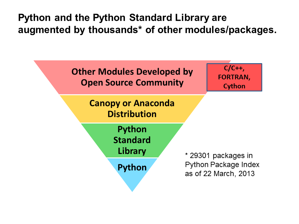
All Python installations include the bottom two layers. (Anyone who has worked with C++ knows that C++ would be almost useless without the C and C++ Standard Libraries. The same is true of Python and the Python Standard Library). If one intends to use Python in even the most elementary scientific or engineering applications, one is likely to need at least the NumPy, SciPy, and matplotlib packages:
NumPy provides support for multi-dimensional arrays and matrices, as well as a large library of high-level mathematical functions for performing array operations.
SciPy builds on NumPy, providing functions for interpolation, linear algebra, numerical integration, Fast Fourier Transforms (FFTs), image processing, optimization, root finding, special functions, statistics, and more.
matplotlib allows one to easily generate high-quality 2-D plots (line plots, scatter plots, contour plots, etc.), 3-D plots (e.g., wire frame plots), and maps of the Earth (using any of a variety of projections) with many types of overlays.
Beyond Canopy Free and Anaconda, there is a wealth—perhaps one should say plethora—of open-source Python modules and packages available through the Python Package Index and other sources on the web, including this site. (The quality of open source software varies, and some packages are supported poorly or not at all, so some care is advised).
Lastly, it is worth mentioning that Python can "wrap" code written in C/C++ and Fortran. This is important for leveraging existing/legacy code, and in some cases for obtaining better runtime performance than would be possible with pure Python.
As the inverted pyramid shape suggests, the number and variey of available
packages increases dramatically as one works one's way up to the yellow and pink
layers. But, at the same time, the quality of code and the quantity and quality
of user documentation tend to decrease commensurately.
One of the great strengths of Python/NumPy is the variety of available data
types, including both "ordinary" data types such as bool,
int, float, complex, str
(string), and so on, and container types such as list,
tuple, dict, set, and array.
Choosing the correct data type/data structure for any given application is
important because the wrong choice may lead to inefficient use of the CPU,
inefficient use of memory, or even wrong results.
Python's list is a container that stores an ordered sequence of
items of arbitrary types; factors that tend to make this data structure a good
choice include the following:
The number of items to be stored grows and/or shrinks over time.
Any insertions and deletions changes occur mainly at or near the high-index end of the list.
The items to be stored do not all have the same type, e.g., one needs to store a mix of integers, strings, and floats.
The list object has append and pop
methods that allow one to efficiently add and remove items from the end of a
list.
In the following example (what is shown is interactive input and output from
an IPython
session), I create a list that stores an integer, a float, a string, and a
nested list containing two integers. I then access selected items. Note that
indexing (of lists, arrays, and so on) always begins at zero, and that we can
use negative indices, which count backwards from the end.
In [1]: x= [3, 4.4, 'dog', [1,2]]

In [2]: x[0]
Out[2]: 3

In [3]: x[-1][1]
Out[3]: 2
As shown in the following example, a list may be extended via
the append method, which adds a single item on the end, or via the
+= operator, which appends all of the items from the
list to the right of the operator.
In [1]: x= []

In [2]: id(x)
Out[2]: 155900232L

In [3]: x.append(0)

In [4]: x
Out[4]: [0]

In [5]: x+= [1, 2, 3]

In [6]: x
Out[6]: [0, 1, 2, 3]

In [7]: id(x)
Out[7]: 155900232L
Results from the id function confirm that the length-4
list is the same object as the original empty (length-0)
list, i.e., x begins at the same address in memory.
One can insert an item into a list at any position using the
insert method, as shown below:
In [1]: x= [1, 2, 3]

In [2]: x.insert(0, 4)

In [3]: x.insert(1, 5)

In [4]: x
Out[4]: [4, 5, 1, 2, 3]
The underlying implementation of the list is an array of
pointers that is automatically resized as needed, e.g., when the array needs to
grow, a new array is allocated, values are copied to the new array, and the
memory associated with the old array is deallocated. (In the C implementation of
Python's list data structure, the
growth factor is 9/8).
All of this happens behind the scenes.
When an item is inserted at the front of a list, all existing
pointers must shift one position to the right, and a pointer to the new item can
then be stored at the front. There is thus a potentially huge performance
difference between inserting an item at the front versus appending to the end.
In the following example, I perform timing tests to evaluate how much CPU time
is required to add 200,000 items to an initially empty list, first by appending
to the end, and then by inserting at the front.
In [1]: import timeit

In [2]: timeit.repeat(stmt="x.append('dog')", setup="x=[]", repeat=1, number=200000)
Out[2]: [0.01923688750270003]

In [3]: timeit.repeat(stmt="x.insert(0, 'dog')", setup="x=[]", repeat=1, number=200000)
Out[3]: [13.920384560481637]
The number in square brackets represents the CPU consumption in seconds. Note that inserting at the front requires over 700 times as much CPU. This discrepancy would be even greater if we continued to grow the lists.
The collections module, which is part of the Python Standard
Library, includes a list-like container called deque that supports
efficient appends and pops on both ends.
tuple is a container that, like a list,
stores items of arbitrary types. A literal tuple is enclosed by
parentheses. Because parentheses are also used for controlling the order of
evaluation in expressions, one must put a comma immediately before the closing
parenthesis in a length-1 literal tuple to avoid ambiguity.
The following example shows that one can access any item of a
tuple via indexing, but items cannot be replaced.
In [1]: x= (1, 2, 3)

In [2]: x[0]
Out[2]: 1

In [3]: x[0]= 4
-----------------------------------------------------------
TypeError: 'tuple' object does not support item assignment
There is no append method for tuples. One can use the
+= operator, but this creates a new tuple object.
In [1]: x= (0,)

In [2]: id(x)
Out[2]: 39747656L

In [3]: x.append(5)
AttributeError: 'tuple' object has no attribute 'append'

In [4]: x+= (1, 2, 3)

In [5]: x
Out[5]: (0, 1, 2, 3)

In [6]: id(x)
Out[6]: 155544960L
In the above example, the results from id confirm that the
length-4 tuple is a different object from the original length-1
tuple, i.e., the new x begins at a different address
in memory, and the memory that held the original x has been
released. (Because Python is dynamically-typed, the object name, type, and other
meta-data must be stored, with the consequence that any Python object—even
a length-0 tuple—occupies memory).
One would at this point be entitled to suspect that the tuple is
simply a cripled version of the list. The Section on "Mutable and
Immutable Objects" below will explain why tuples are necessary.
When the order of the items is not important and no item appears more than
once, the set data structure is often a better choice than the
list. The Python set supports all of the standard
operations of mathematical set theory, including union, intersection,
difference, and testing for membership.
In the following example, I create a set containing three items,
test for membership of an item that is not present, add the missing item, and
then test again.
In [1]: x= set(['cat', 'dog', 3])

In [2]: x
Out[2]: {3, 'cat', 'dog'}

In [3]: 'fish' in x
Out[3]: False

In [4]: x.add('fish')

In [5]: x
Out[5]: {3, 'cat', 'dog', 'fish'}

In [6]: 'fish' in x
Out[6]: True
Because the Python set is implemented using a hash table, the
time to insert an item or test for the presence of an item is independent of the
number of items stored. The time to insert an item or test for the presence of
an item at a random position in a list is essentially proportional to the length
of the list. In computer science terminology, when required CPU time for an
operation is essentially independent of the size of a data structure, this is
known as O(1) performance, while the situation where required CPU time is
proportional to size is known as O(n) performance. (More precisely,
f(n)= O(g(n)) means that f(n) is overbounded by a constant
multiple of g(n) in the limit of large n).
I wrote a small Python script that loads a
181,000-word spelling dictionary, stores it as either a list
or a set, and measures the time to look up the word
zeitgeist in each. (I picked this word because it appears near the end
of the dictionary). The source code follows:
import timeit

setup= """
with open('large.txt', 'r') as FILE:
    words= [word.rstrip() for word in FILE]"""

t_list= timeit.repeat(stmt="'zeitgeist' in words", setup=setup, repeat=1, number=2000)

setup= """
with open('large.txt', 'r') as FILE:
    words= set([word.rstrip() for word in FILE])"""

t_set= timeit.repeat(stmt="'zeitgeist' in words", setup=setup, repeat=1, number=2000)

print("Ratio= %.1f" % (t_list[0] / t_set[0]))
The result shows that runtime performance is over 50,000 times faster with
the set! The secondary moral of this story is that the difference
between O(1) and O(n) performance is substantial if n is
sufficiently large.
Support for arrays is not part of Python itself, but is provided through the
widely-used NumPy library. An array (type=numpy.ndarray) can have
any number of dimensions. (Unlike Matlab, which requires that an array have at
least two dimensions, a NumPy array can be 1-D or even 0-D; a 0-D array is more
or less equivalent to a scalar). A given array typically stores elements that
are all of the same type (and size), but we will see that that an array can also
store items of multiple types.
dtypeAn array has a dtype attribute that specifies the type or
types of data that the array stores. There are several ways to create an array.
Three of these are shown in the example below.
In [1]: from numpy import array, empty, zeros

In [2]: x= array([1, 2, 3])

In [3]: y= zeros(shape=(3,4), dtype='f8')

In [4]: z= empty(shape=y.shape, dtype='object')

In [5]: x.dtype
Out[5]: dtype('int32')

In [6]: y.dtype
Out[6]: dtype('float64')

In [7]: z.dtype
Out[7]: dtype('O')
The x array is created via the numpy.array
function, which accepts a list containing the data with which the
array is to be initialized. In this case, x is a 1-D array, but we
could have created a multi-dimensional array using nested lists. Because we
haven't specified the dtype of the array, it is determined from the
contents of the list.
The y array is created via the numpy.zeros
function. The first argument of this function, which must be either an integer
or a tuple of integers, specifies the dimensionality of the array.
The second argument specifies the dtype.
The z array is created via numpy.empty, which
allocates a block of memory without initializing it. (The memory retains
whatever happened to be left there). Eliminating the array initialization
overhead makes numpy.empty a very fast way to create a large array.
When storing a fixed-length, ordered sequence of objects all having the same
type (e.g., 32-bit signed integers or 64-bit floats), a one-dimensional array is
generally more appropriate than a list because (A) memory is
utilized more efficiently and (B) operations such as calculating a sum or an
average that operate on the entire data structure can be performed far more
efficiently.
An array having dtype='object' stores items of arbitrary types,
and is thus comparable to a list, except that the array size is
fixed.
While Matlab arrays always have at least two dimensions, a NumPy array may have one or even zero dimensions. (A zero-dimensional array is equivalent to a scalar).
Matlab uses 1-based indexing, i.e., the lowest value of any index is 1. Python, like most other computer languages, uses 0-based indexing.
When one attempts to store a value at an index beyond the current limits of a Matlab array, the array is automatically resized. This can be convenient, but can also have a substantial impact on runtime performance and usually masks a poor application design. If one attempts to write beyond the end of a NumPy array, an exception (fatal error) is raised. One can manually resize a NumPy array, e.g., by adding rows and/or columns, but this never happens automatically.
With Matlab, if one adds a complex value to one element of a float
array, the entire array is converted to complex. Once a Numpy array has been
created, its dtype does not change, and adding a complex value to
a float array will generate a message warning the user that the imaginary part
of the complex number has been discarded. One can manually change the
dtype of a NumPy array, but this never happens automatically.
In some situations, Python-level looping over arrays is unavoidable, but whenever explicit looping can be and is avoided, code tends to run much faster. The following timing tests demonstrate this.
In [1]: import timeit

In [2]: timeit.repeat(stmt="for i in xrange(200000):\n   x[i]='dog'", \
  setup="import numpy;x=numpy.empty(200000, dtype='object')", repeat=1, number=1)
Out[2]: [0.012643140342959214]

In [3]: timeit.repeat(stmt="x[:]='dog'", \
  setup="import numpy;x=numpy.empty(200000, dtype='object')", repeat=1, number=1)
Out[3]: [0.0004944922427512211]
In the second example, explicit looping is avoided by assigning to a slice that includes the entire array. (Looping still occurs, but at the level of compiled C, which is extremely fast).
Comparing to the timing result in the section on lists, we see that the array is somewhat faster than the list. But, this difference is small compared to the benefit from avoiding Python-level looping.
In a NumPy structured array, each element has multiple fields, much like in a relational database. When creating a structured array, one can choose the data types (e.g., 32-bit integer, 64-bit float, etc.) of the different fields independently, and each field is typically assigned a mnemonic name.
To store an association or mapping between pairs of items, the natural
choice is a dictionary (dict). In Computer Science, these are
often called
hash tables. The following example demonstrates the use of a
dict:
In [1]: sound= {'cat':'meow', 'dog':'woof', 'mouse':'squeak'}
In [2]: sound['cat']
Out[2]: 'meow'
In the above dictionary, 'cat', 'dog', and
'mouse' are keys, and 'meow',
'woof', and 'squeak' are the corresponding
values. This example is not very impressive, but Python dictionaries are
extremely flexible—there are no type restrictions on the values, and only
mild type restrictions on the keys (see below).
Under the hood, checking whether a given key exists in a dictionary requires hashing the key and then using the result as an index into an array. Thus, the time to check whether a given key exists in a dictionary containing n key-value pairs is essentially O(1). Dictionaries are also extremely convenient. Bottom line: The power of Python dictionaries cannot be overstated.
For the sake of complete disclosure: The O(1) claim is not exactly true. A dictionary that will contain only 10 keys can use very small keys, while a dictionary that will contain 100 billion keys must use larger keys. (And, the time to hash a key is roughly proportional to the length of the key). Also note that the time to check whether a given value appears in a dictionary is O(n).
Python/NumPy lists, dictionaries, sets, and arrays are mutable, meaning that the contents of the object can be modified. In the case of lists, this means that one can replace a specific item, remove an item, or append a new item without rebuilding the entire object. User-defined classes are also mutable; at any time, new attributes can be added and attribute-value pairs can be modified.
Strings and tuples (and, of course, such non-container types as integers and floats) are immutable; contents of these objects cannot be modified, although one can always destroy the object and create a new one.
The following example shows what happens if one attempts to modify the contents of a string:
In [1]: x='tops'
In [2]: x[0]= 'o'
TypeError: 'str' object does not support item assignment
Immutable types are necessary mainly because Python implements sets and dictionaries using hash tables; allowing hash table keys to be mutable would create complex problems. (If the contents of the key object changed, the mapping from keys to indices would no longer be valid). Thus, objects that are stored in sets or used as dictionary keys must be immutable.
The following example shows what happens if one attempts to violate these rules:
In [1]: x=set()
In [2]: x.add([1, 2])
TypeError: unhashable type: 'list'

In [3]: x={}
In [4]: x[[1, 2]]= 'oops'
TypeError: unhashable type: 'list'
There are situations where one needs to construct a key as a collection of
sub-keys; tuples provide such a mechanism, without the issues that would arise
if one allowed the use of mutable containers such as lists as keys.
Mutability is simultaneously convenient and dangerous. When one copies a mutable object by assignment, Python creates a reference rather than a true copy. Because the copy and the original are one and the same object, modifying one modifies the other, as the following example shows.
In [1]: x= [1, 2, 3]

In [2]: y= x

In [3]: y[0]= 0

In [4]: x
Out[4]: [0, 2, 3]
One can make a true copy of a list or other mutable object using
copy.deepcopy, as shown in the following example:
In [1]: import copy

In [2]: x= [1, 2, 3]

In [3]: y= copy.deepcopy(x)

In [4]: y[0]= 0

In [5]: x
Out[5]: [1, 2, 3]

In [6]: y
Out[6]: [0, 2, 3]
If a mutable object is passed to a function that modifies the object, the calling program's copy of the object is also modified, as shown in the following example. (When a function has such side effects, its doc string should contain a suitable warning).
In [1]: def f(x):
   ...:     x.append(x[0])
   ...:     return sum(x)
   ...:

In [2]: z= [1, 2, 3]

In [3]: f(z)
Out[3]: 7

In [4]: z
Out[4]: [1, 2, 3, 1]
We can easily prevent such side effects, as shown below.
In [5]: def f(x):
   ...:     x= x + [x[0]]
   ...:     return sum(x)
   ...:

In [6]: z= [1, 2, 3]

In [7]: f(z)
Out[7]: 7

In [8]: z
Out[8]: [1, 2, 3]
The second statement of the function definition creates a new variable
x that exists only within the namespace of the function, i.e., it
is distinct from the x in the namespace of the calling program.
Nested data structures can serve a variety of purposes. Suppose that one wants to store a directed graph. This could be done in any of several ways. A dictionary of lists of strings is one possible choice:
In [1]: g['a']= ['b', 'd']

In [2]: g['b']= ['a', 'c']

In [3]: g['d']= ['a', 'b']

In [4]: g
Out[4]: {'a': ['b', 'd'], 'b': ['a', 'c'], 'd': ['a', 'b']}
If we are working with a large graph and need to frequently test whether
there is a link from one node to another, a dictionary of sets of strings would
be more efficient that the dictionary of lists of strings. Another option would
be a set of length-2 tuples of strings.
A Python class allows one to define an object type, including methods that can operate on the data stored in instances of that object. (As in other OOP languages, methods can be thought of as class-specific functions). Once a class has been defined, one can create as many instances as desired. Each instance stores its own data. Each item of data within a class has a name; these attributes are typically the same across all instances of a given class, but not necessarily so. Methods are common to all instances of a given class.
Python OOP has three main selling points:
There is considerable power and flexibility (not quite as much as in C++, but enough for the vast majority of applications).
Defining a class in Python typically requires much less code than would be needed in C++ and most other languages.
Unlike in Matlab, Python classes are not tied to the file system folder structure.
Each class must contain at least one method, known as the
constructor; this method, which has the special name
__init__, is invoked when a new instance of the class is created.
The following example defines a simple class that can be used as a substitute
for the C struct, with the added flexibility that attributes-value
pairs can be added and removed at any time. This object is equivalent to a
Python dictionary, but the data are accessed as attributes, e.g., using the
notation x.a rather than x['a'].
class Struct(object):
   """
   This simple class allows one to create an object whose attributes are
   initialized via keyword argument/value pairs.  One can add and remove
   attributes as needed later.
   """
   def __init__(self, **kwargs):
      self.__dict__.update(kwargs)

   def __repr__(self):
      """
      Product a string representation of the object.
      """
      return 'Struct(' + \
        ', '.join(['%s=%r' % kv for kv in self.__dict__.items()]) + ')'

   def pop(self, k):
      """
      Remove an attribute key-value pair and return the value.
      """
      try:
         return self.__dict__.pop(k)
      except:
         return None
In the following IPython session, two instances of the class are created. An
attribute-value pair is added to the y object after creation.
In [1]: x= Struct(a=5, b='bat')

In [2]: y= Struct(a=4, c='cat')

In [3]: y.d= 'dog'

In [4]: x
Out[4]: Struct(a=5, b='bat')

In [5]: y
Out[5]: Struct(a=4, c='cat', d='dog')
goodbye.pyAlmost every programming class in any language begins by having the students
write a program that displays "Hello World!" Since such a program is not
particularly instructive, I'd like to end this tutorial with a simple program
called goodbye.py. The source code listing follows:
# This program displays "goodbye" in a randomly selected language.

import numpy

def pick_one_at_random(L):
   """
   This function accepts a list L and returns a randomly-selected item from that
   list.  Note that `numpy.random.randint(n)` returns a random integer from the
   set {0, 1, 2, ..., n-1}.
   """
   return L[numpy.random.randint(len(L))]

print(pick_one_at_random(['Adios', 'Aloha', 'Arrivederci', 'Au Revoir',
  'Auf Wiedersehen', 'Ciao', 'Do svidanja', 'Farvael', 'Goodbye',
  'Hasta La Vista', 'Lehitra\'ot', 'Salut', 'Sayonara', 'Vale']))
Although very simple, this program illustrates certain features common to most Python programs. Here are a few things to note:
def statement followed by an (optional) triple-quoted
doc string. (A doc string is similar to a comment in some respects, but
the doc string at the top of a function is parrotted back by the IPython
interactive environment when you ask for help information for that function). It
is good practice to write a header comment for each
module
(source code file) and a doc string for each function, class, or method to
explain its purpose and how to use it; in the long run, this practice will save
you time when you revisit code that you haven't looked at for a while, and it
will save even more time for anyone else who works with your code. (The module
header comment may also be a tripled-quoted doc string; this is more convenient
than prefacing each line of a multi-line comment with a pound sign).import
statement. This statement loads the specified module, makes all variables and
functions defined in that module available to the program that performs the
import. The typical Python program will import from multiple modules.def statement indicates the start of a function definition.
The body of the function consists of the indented lines following the
def statement. The end of the function (like the end of any other
block) is indicated by the return of the level of indentation to that of the
statement—in this case the def statement—that opened
the block.main function. The "main program" consists of all
code outside the function definition—namely, the import
statement and the print statement.print function is an invocation of the
pick_one_at_random function that we defined earlier in the program,
and also makes use of a literal/anonymous list, i.e., a list that is not stored
in a named variable.Click on the following link to run an expanded version that includes more languages and also identifies the language.
"Learn Python the Hard Way, URL= http://learnpythonthehardway.org/book: This tutorial might more aptly be called "Learn Python the Slow Way", but it is incredibly thorough, and a good resource for those without experience in other programming languages.
Norm Matloff's Python tutorial, URL= http://heather.cs.ucdavis.edu/~matloff/python.html: This tutorial is somewhat dated, but very readable, and a good choice if you are looking for something short and to the point.
Python Introduction, Resources and FAQs, URL= http://www.whoishostingthis.com/resources/python: This page is mainly a collection of links to other Python resources.