Prime Numbers and Their Statistical Properties

Dr. Phillip M. Feldman

Introduction

A prime number is an integer greater than 1 that is divisible only by itself and one.

This simple definition leads to many interesting properties. There are two properties of prime numbers, and of their relationship to the integers, that are of special importance:

(1) Every integer greater than 1 can be written as a product of prime numbers, and, except for the order of the factors, this can be done in only one way.

For example, 6 can be written as 2 · 3 or 3 · 2; there is no other way to express 6 as a product of prime factors.

(2) The Prime Number Theorem (PNT) states, roughly speaking, that the density of prime numbers diminishes logarithmically. A more precise statement of this is that if one randomly selects an integer i from the set {1, 2, ..., N}, the probability that i is prime tends to

in the limit of large N. [ln(N) is the natural logarithm of N.]

One implication of (2) is that there is no largest prime number. (One can establish this without recourse to the PNT. Assume that there is a largest prime, multiply all prime numbers together, and add or subtract one. The result cannot be divided by any prime, and must itself thus be prime, contradicting the hypothesis that there is a largest prime number).

Another implication of (2) is that in the vicinity of a large integer N, the average spacing between primes should be tend to

for large N. Vicinity is a bit vague and not easily clarified. Suffice it to say that the interval over which we examine the average spacing must be large compared to the average spacing (to eliminate small sample variation) but still small compared to N.

Let's use the PNT to find the number of primes in the interval from 1980 to 2020, inclusive. The theorem says that we should expect 41 / log(1000)= 5.9 primes. If you have access to a computer with the Python interpreter, you can easily determine the actual number as follows. Download the primes.py module (see link at end of this page), open ipython, and issue the following commands:

   from numpy import *
   from primes import *
   P= array(find_primes(200))
   ((980<=P) & (P<=1020)).sum()

The interpreter should display a result of 6. Not bad! Actually, predictions of the number of primes to be found in a short interval are typically not this accurate because the distribution of primes is highly irregular.

Prime numbers have been a subject of mathematical inquiry for over 23 centuries. They have fascinated professional mathematicians, amateurs, and to some extent, even the public at large. Some properties of prime numbers are difficult to prove, and there are many conjectures involving prime numbers that are almost certainly true but that have resisted attempts at proof for hundreds of years.

Although the prime number sequence is of course deterministic, the primes exhibit some interesting statistical behavior. This may be surprising, but there are in fact many settings where deterministic sequences exhibit small- or large-scale behavior that not only appears to be random, but that is indistinguisable from true randomness. We will return shortly to the subject of randomness in the prime numbers.

Although prime numbers are often thought of as belonging to the domain of recreational mathematics, there are many practical applications. Here are a few examples:

The RSA algorithm for public-key cryptography depends on the computational difficulty of factoring a product of two large prime numbers.
The Mersenne Twister algorithm for generating pseudorandom numbers—the best such algorithm currently available—has a connection to the Mersenne primes.

Some interesting and perhaps surprising properties of prime numbers can be explored without recourse to advanced mathematics. Two examples that I present below make use of elementary statistical concepts, but otherwise require essentially no math background. Generating the results required nothing more than a laptop computer, a Python interpreter, and some knowledge of programming.

Twin Primes and Prime Triples

Twin primes are pairs of primes of the form (p, p+2). The first few twin primes are (3,5), (5,7), (11,13), and (17,19). A famous conjecture that has never been proven states that there are infinitely many twin primes.

In 2008, PBS's NOVA scienceNOW posted a video of a song about the twin prime conjecture. The song is rather cute, but obscures more than it illuminates. In particular, the lyrics imply that prime numbers always occur in pairs, which is of course not true. Aside from 2, 23 is the first prime number that is not a twin prime.

There is in some sense nothing special about twin primes. Many other constellations of primes can be defined, including pairs that differ by 4, or by 6, and so on. Primes also occur in groups of more than two. I will use the term prime triple to refer to a group of three primes such that the largest and smallest differ by no more than 6. With the exception of (2, 3, 5) and (3, 5, 7), all prime triples are of one of two forms:

Form 1: p, p+2, p+6
Form 2: p, p+4, p+6

Note that (3, 5, 7) is the only prime triple of the form (p, p+2, p+4) because in any such triple, at least one of the three numbers must be divisible by 3. The following table lists the first 20 and selected larger prime triples (large integers are written without commas so that the rate of growth can be judged from the lengths of the numbers):

       1:          2          3          5
       2:          3          5          7
       3:          5          7         11
       4:          7         11         13
       5:         11         13         17
       6:         13         17         19
       7:         17         19         23
       8:         37         41         43
       9:         41         43         47
      10:         67         71         73
      11:         97        101        103
      12:        101        103        107
      13:        103        107        109
      14:        107        109        113
      15:        191        193        197
      16:        193        197        199
      17:        223        227        229
      18:        227        229        233
      19:        277        281        283
      20:        307        311        313
     100:       7873       7877       7879
    1000:     247603     247607     247609
   10000:    5037913    5037917    5037919
  100000:   88011613   88011617   88011619
 1000000: 1385338061 1385338063 1385338067

Strictly speaking, the numbers of primes, primes pairs, and prime triples are all the same because all are countably infinite. (A set is countably infinite if there is a one-to-one mapping between its elements and the integers; see the Wikipedia article referenced below for further discussion). But, in another sense, there are far more primes than prime pairs, and far more prime pairs than prime triples. The 3 millionth prime number is 49,979,687; comparing this with the millionth prime triple in the above table, we can see that only a tiny percentage of the primes between 1 and 1,385,338,067 occur in prime triples.

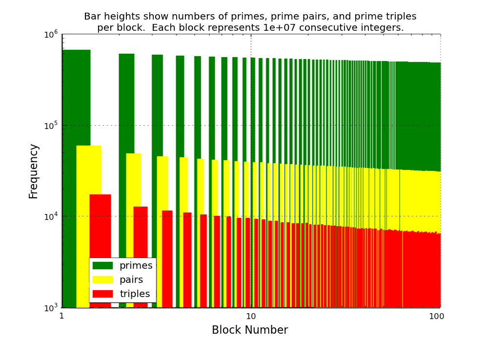
Figure 1 below displays the frequencies of primes, primes pairs, and prime triples among the first billion integers. Each set of three bars represents the counts from a block of 10 million consecutive integers. Note that the frequency of primes pairs diminishes faster than that of primes, while the frequency of prime triples diminishes even faster. (The y-axis has a logarithmic scale, so the increasing distances between the tops of the yellow and green bars and between the red and yellow bars indicates that the ratios are increasing). Thus, the tendency of prime numbers to cluster together gradually diminishes, i.e., the primes become increasingly isolated.

Figure 1: Frequencies of Primes, Twin Primes (Pairs), and Prime Triples Among the First Billion Integers

The results shown in the above graph strongly suggest that the asymptotic fractions of primes occurring in prime pairs and in prime triples are both zero. (Note that this is not a proof. A picture may sometimes be worth a thousand words, but not in mathematics, where nothing can be proven with a picture. Furthermore, general results cannot be proven by any number of examples as long as the possibility of a counterexample remains). Although the primes do tend to become more isolated, prime pairs, prime triples, and larger clusters of primes occur infinitely often.

The Poisson Distribution and Poisson Random Process

The Poisson distribution is one of the most important discrete distributions. For definitions and background, see http://en.wikipedia.org/wiki/Poisson_distribution or http://math.wikia.com/wiki/Poisson_distribution. The Poisson distribution family has the following rare property: The sum of any two independent Poisson random variables yields another Poisson random variable. (The normal distribution family shares this property, i.e., the sum of any two independent normal random variables yields another normal random variable). It can be proven that the Poisson distribution tends to a normal distribution in the limit as its mean becomes large.

The stationary (homogeneous) Poisson process is a random function of time that counts events of some type, with the properties that (A) the number of events in any interval has a Poisson distribution with mean proportional to the length of the interval, and (B) the numbers of events in non-overlapping intervals are independent random variables. The constant of proportionality in (A) is called the rate of the process. The nonstationary (inhomogeneous) Poisson process is a generalization that allows the rate to be a function of time rather than a constant; in this case, the expected number of arrivals in an interval becomes the integral of the rate function over that interval. Note that properties (A) and (B) are consistent with the aforementioned property of sums of independent Poisson random variables.

Poisson processes are used for modeling a wide variety of real-world phenomena; three of the best known modeling applications are:

radioactive decay. The Poisson process arises because atoms decay independently.
shot noise in analog electronic devices. Electric charge is quantized; when the flow of electrons is sufficiently small, as through the junction of a reverse-biased diode, the noise associated with individual electrons transiting the junction can be significant.
starting times for telephone calls handled by a large switch. The Poisson process arises because a large number of people make independent decisions about when to pick up the phone.

Connection Between Primes and the Poisson Distribution

There is a surprising connection between primes and the Poisson distribution.

The next several plots are histograms of counts of prime numbers from equal-sized blocks of consecutive integers. (Each plot was generated using equal-sized blocks, but the block size is differs from one plot to the next, as noted in the plot titles). A new block starts whenever an integer n is reached such that n mod b= 1, where b is the block size. In each plot, the green bars show the counts of prime numbers, while the blue bars show the corresponding Poisson probability mass function (PMF). The mean of the Poisson distribution has been chosen to match the sample mean of the data. (The scaling makes the two sets of bars have the same total area).

Figure 2 was generated with a block size b= 7 and initial integer n=2. (This block size was chosen to produce a mean number of primes per block between 1 and 2). Despite the ample size of the sample, the Poisson distribution does not appear to be a good fit to the data.

Figure 2: Comparison of Prime Frequencies and Poisson Distribution for Initial Integer=2, Small Block Size

The data for Figure 3 was generated by increasing the block size, which increases the mean of the Poisson distribution. Notice that the distribution is beginning to converge to the normal curve. (Recall that the Poisson tends to a normal limit as its mean becomes large).

Figure 3: Comparison of Prime Frequencies and Normal Distribution for Initial Integer=2, Larger Block Size

Figure 4 was created by specifying a value of 22000 for the initial integer. This value was chosen to produce an average spacing of 10 between consecutive prime numbers. Note that the fit between the data and the Poisson distribution is no better than what was obtained with an initial integer of 2.

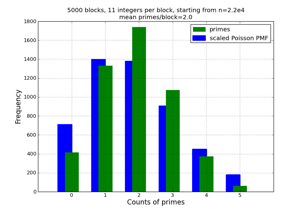
Figure 4: Comparison of Prime Frequencies and Poisson Distribution for Initial Integer=22000

Figure 5 was created by specifying a value of 2.7e43 for the initial integer. This value was chosen to produce an average spacing of 100 between consecutive prime numbers. Note that we have finally obtained a reasonably close fit between the data and the Poisson distribution.

Figure 5: Comparison of Prime Frequencies and Poisson Distribution for Initial Integer=2.7e43

The above statistical results suggest two questions:

Why does the prime number sequence exhibit Poisson behavior? The proof of this requires some difficult math; I hope to eventually add a discussion of some of the ideas in the proof to this web page.
Why does the Poisson behavior emerge only for relatively large integers? Aside from small-sample variation, I believe that there are two explanations for discrepancies between the histograms and the scaled Poisson distribution:
- The underlying distribution of the data is shifting from one block to the next as the frequency of primes diminishes. For any fixed block size, we can see from the Prime Number Theorem that this change should be initially rapid, but gradually slowing.
- For small integers, the discrete step between one integer and the next is significant compared to the average increment between one prime number and the next. In a Poisson process, the time between one 'arrival' and the next must be an exponential random variable, which has a continuous distribution, and thus cannot be constrained to the integers.

For both radioactive decay and prime numbers, the expected (average) number of 'events' per unit time diminishes, and both processes are thus non-stationary. The rate laws are of course different. The rate of radioactive decay diminishes exponentially (hence the term half life), while the rate at which prime numbers appear decays much more slowly (see the discussion of the Prime Number Theorem above). This difference is important: If one is willing to wait long enough (long enough might make the present age of the universe seem insignificant) any chunk of radioactive material will eventually emit its last particle. The prime numbers, on the other hand, go on forever.

References

(1) Mathworld article on twin primes

(2) This Wikipedia article defines the term 'countably infinite'.

(3) primes.py: This Python module contains functions for performing various calculations involving prime numbers, including primality testing, prime factorization, and the like. All numerical results presented in this article were generated using the Enthought Python distribution and the primes.py module.

Last update: 16 May, 2020